Time series handling

This Notebook shows a general calculation stream for time series. You will see how to * read in time series * plot the data in time and frequency domain * filter the time series with a bandpass filter * remove spikes using running statistics * calculate and plot the rainflow matrices of the time series * combine the PSD to an envelope PSD.

If you have any question feel free to contact us.

[1]:

import numpy as np
import pandas as pd

import pylife.utils.histogram as psh
import pylife.stress.timesignal as ts
import pylife.stress.rainflow as RF
import pylife.stress.rainflow.recorders as RFR
import pickle

import pyvista as pv

import matplotlib.pyplot as plt
from mpl_toolkits.mplot3d import Axes3D
from matplotlib import cm
import matplotlib as mpl

from scipy import signal as sg

# mpl.style.use('seaborn')
mpl.style.use('bmh')
get_ipython().run_line_magic('matplotlib', 'inline')

some functionality to plot the rainflow matrices

[2]:

from helper_functions import plot_rf

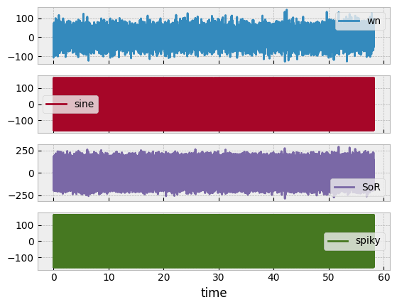
Time series signal

import, filtering and so on. You can import your own signal with

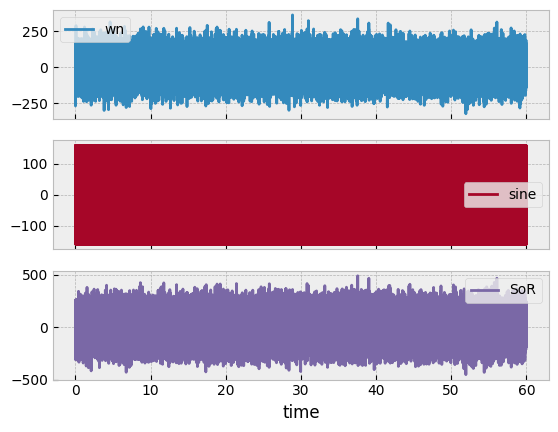
and so on. Here we define a white noise, a sine and a sine on random signal.

[3]:

np.random.seed(4711)
sample_frequency = 1024
t = np.linspace(0, 60, 60 * sample_frequency)
signal_df = pd.DataFrame(data = np.array([80 * np.random.randn(len(t)),
                                          160 * np.sin(2 * np.pi * 50 * t)]).T,
                         columns=["wn", "sine"],
                         index=pd.Index(t, name="time"))
signal_df["SoR"] = signal_df["wn"] + signal_df["sine"]
signal_df.plot(subplots=True)

[3]:

array([<Axes: xlabel='time'>, <Axes: xlabel='time'>,
       <Axes: xlabel='time'>], dtype=object)

../_images/demos_time_series_handling_5_1.png

[4]:

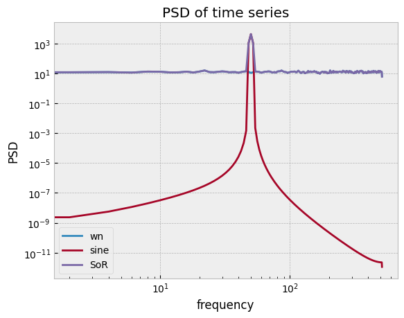
ts.psd_df(signal_df, NFFT = 512).plot(loglog=True, ylabel="PSD", title="PSD of time series")

[4]:

<Axes: title={'center': 'PSD of time series'}, xlabel='frequency', ylabel='PSD'>

../_images/demos_time_series_handling_6_1.png

Filtering

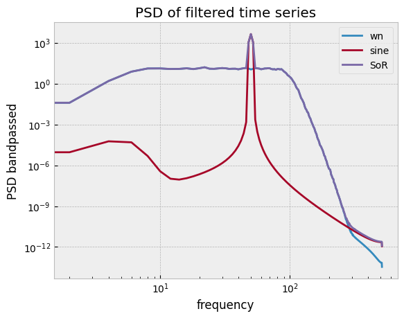
We are using a butterworth bandpass filter from scipy.signal to filter the time series.

[5]:

f_min = 5.0    # Hz
f_max = 100.0  # Hz

[6]:

bandpass_df = ts.butter_bandpass(signal_df, f_min, f_max)

df_psd = ts.psd_df(bandpass_df, NFFT = 512)
df_psd.plot(loglog=True, ylabel="PSD bandpassed", title="PSD of filtered time series")

[6]:

<Axes: title={'center': 'PSD of filtered time series'}, xlabel='frequency', ylabel='PSD bandpassed'>

../_images/demos_time_series_handling_9_1.png

Running statistics

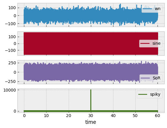
First we create a spike in our existing data set

[7]:

bandpass_df["spiky"] = bandpass_df["sine"] + 1e4 * sg.unit_impulse(signal_df.shape[0], idx="mid")
bandpass_df.plot(subplots=True)

[7]:

array([<Axes: xlabel='time'>, <Axes: xlabel='time'>,
       <Axes: xlabel='time'>, <Axes: xlabel='time'>], dtype=object)

../_images/demos_time_series_handling_12_1.png

Now we want to clean this spike automatically

[8]:

cleaned_df = ts.clean_timeseries(bandpass_df, "spiky", window_size=1024, overlap=32,
                     feature="maximum", method="remove", n_gridpoints=3,
                     percentage_max=0.05, order=3).drop(["time"], axis=1)

cleaned_df.plot(subplots=True)

Feature Extraction: 100%|██████████| 244/244 [00:00<00:00, 6403.04it/s]

[8]:

array([<Axes: xlabel='time'>, <Axes: xlabel='time'>,
       <Axes: xlabel='time'>, <Axes: xlabel='time'>], dtype=object)

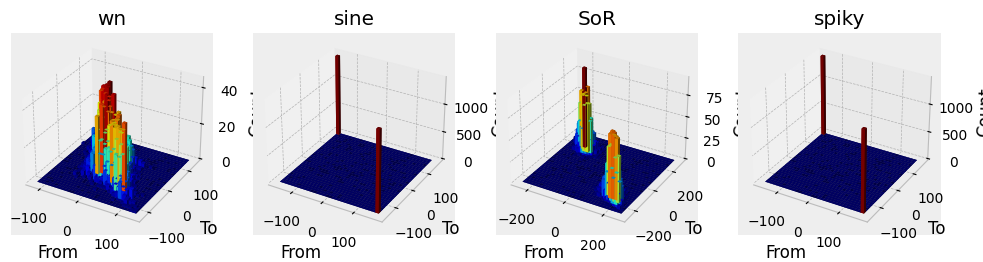
../_images/demos_time_series_handling_14_2.png

Rainflow

The rainflow module in pyLife can be used with different counting methods:

FKM
Three point
Four point enhanced

[9]:

rainflow_bins = 32

[10]:

#%% Rainflow for a multiple time series
recorder_dict = {key: RFR.FullRecorder() for key in cleaned_df}
detector_dict = {key: RF.FKMDetector(recorder=recorder_dict[key]).process(cleaned_df[key]) for key in cleaned_df}
rf_series_dict = {key: detector_dict[key].recorder.histogram(rainflow_bins) for  key in detector_dict.keys()}

[11]:

f = plot_rf(rf_series_dict)

../_images/demos_time_series_handling_18_0.png

[12]:

#%% Now Combining different RFs to one
rf_series_dict["wn + sn"] = psh.combine_histogram([rf_series_dict["wn"],rf_series_dict["sine"]],
                                                  method="sum")
f = plot_rf(rf_series_dict)

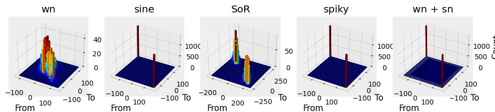
../_images/demos_time_series_handling_19_0.png

You can see the difference of the rainflow matrices of SoR and wn+sn.

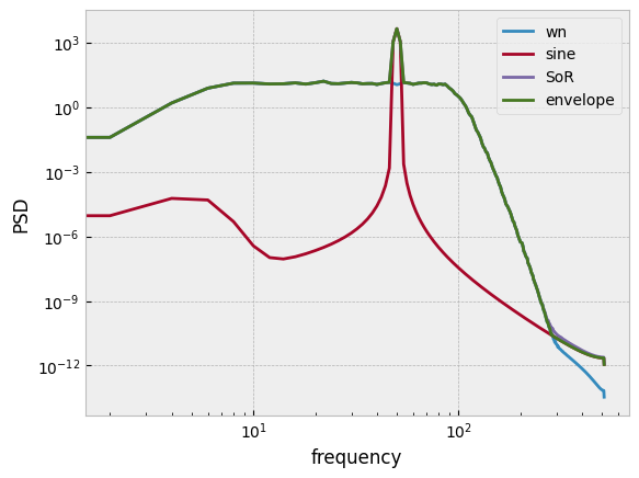
PSD combinig

It is also possible to combine spectra

[13]:

df_psd["envelope"] =  df_psd[["sine", "wn"]].max(axis = 1)
df_psd.plot(loglog=True, ylabel="PSD")

[13]:

<Axes: xlabel='frequency', ylabel='PSD'>

../_images/demos_time_series_handling_22_1.png

Saving

Now we saving the rainflow data into a pickle file. If you want to have an introduction to damage and failure probability calculation, please have a look on the notebook lifetime_calc

[14]:

rf_dict = {k: rf_series_dict[k] for k in ["wn", "sine", "SoR"] if k in rf_series_dict}
%store rf_dict

Stored 'rf_dict' (dict)