Life time Calculation
This Notebook shows a general calculation stream for a nominal and local stress reliability approach.
Overview
Stress derivation
We are starting with the imported rainflow matrices. More information about the time series and loading handlin and the RF generation you can find in the notebook time_series_handling
Mean stress correction
Multiplication with repeating factor of every manoveur
Damage Calculation
Select the damage calculation method (Miner elementary, Miner-Haibach, …)
Calculate the damage for every load level and the damage sum
Calculate the failure probability with or w/o field scatter
Local stress approach
Load the FE mesh
Apply the load history to the FE mesh
Calculate the damage
[1]:
import numpy as np
import pandas as pd
import pickle
from pylife.utils.histogram import *
import pylife.stress.timesignal as ts

import pylife.stress.equistress

import pylife.stress
import pylife.strength.meanstress as MS
import pylife.strength.fatigue

import pylife.mesh.meshsignal

from pylife.strength import failure_probability as fp
import pylife.vmap

import pyvista as pv

import matplotlib.pyplot as plt
import matplotlib as mpl

from scipy.stats import norm

from helper_functions import plot_rf
# mpl.style.use('seaborn')
# mpl.style.use('seaborn-notebook')
mpl.style.use('bmh')
%matplotlib inline
[2]:
%store -r rf_dict
Meanstress transformation
Here we are using the FKM Goodman approach to calculate the meanstress transformation
[3]:
meanstress_sensitivity = pd.Series({
    'M': 0.3,
    'M2': 0.2
})
[4]:
transformed_dict = {k: rf_act.meanstress_transform.fkm_goodman(meanstress_sensitivity, R_goal=-1.).to_pandas() for k, rf_act in rf_dict.items()}
Repeating factor
If you want to apply a repeating factor to your loads you can do it very easily:
[5]:
repeating = {
    'wn': 50.0,
    'sine': 25.0,
    'SoR': 25
}
[6]:
load_dict = {k: transformed_dict[k] * repeating[k] for k in repeating.keys()}
We are calculating a seperat load case, where we summarize the three channels together. Later on we can compare the damage results of this channel with the sum of the other channels.
[7]:
load_dict['total'] = pd.concat([load_dict[k] for k in load_dict.keys()])
[8]:
bins = pd.interval_range(0., load_dict['total'].load_collective.use_class_right().amplitude.max(), 64)
rebinned_dict = {k: rebin_histogram(v.load_collective.amplitude_histogram, bins) for k, v in load_dict.items()}
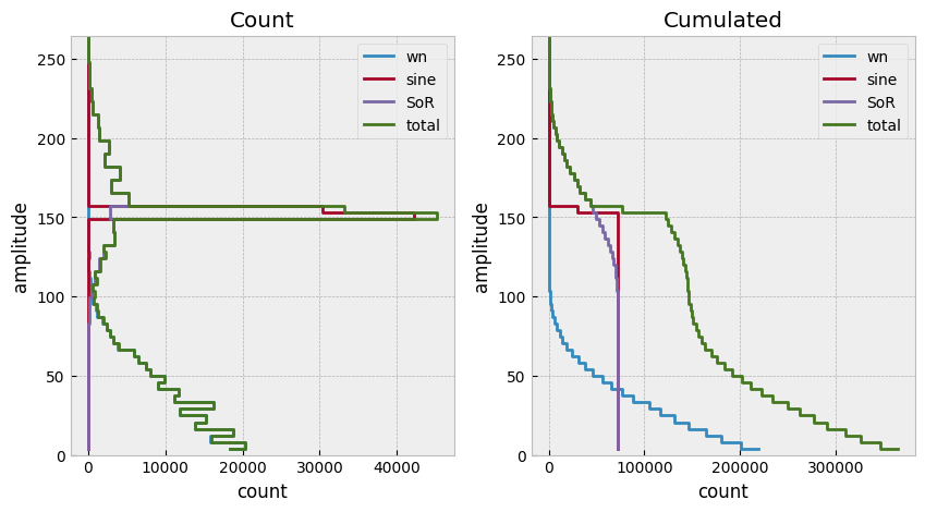
[9]:
fig, ax = plt.subplots(nrows=1, ncols=2,figsize=(10, 5))

for k, v in rebinned_dict.items():
    amplitude = v.index.right[::-1]
    cycles = v[::-1]
    ax[0].step(cycles, amplitude, label=k)
    ax[1].step(np.cumsum(cycles), amplitude, label=k)

for title, ai in zip(['Count', 'Cumulated'], ax):
    ai.set_title(title)
    ai.xaxis.grid(True)
    ai.legend()
    ai.set_xlabel('count')
    ai.set_ylabel('amplitude')
    ai.set_ylim((0,max(amplitude)))
Nominal stress approach
Material parameters
You can create your own material data from Woeler tests using the Notebook woehler_analyzer
[10]:
k_1 = 8
mat = pd.Series({
    'k_1': k_1,
    'k_2' : 2 * k_1 - 1,
    'ND': 1.0e6,
    'SD': 300.0,
    'TN': 12.,
    'TS': 1.1
})
display(mat)
k_1          8.0
k_2         15.0
ND     1000000.0
SD         300.0
TN          12.0
TS           1.1
dtype: float64
Damage Calculation
Now we can calculate the damage for every loadstep and summarize this damage to get the total damage.
[11]:
# damage for every load range
damage_miner_original = {k: mat.fatigue.damage(v.load_collective) for k, v in load_dict.items()}
damage_miner_elementary = {k: mat.fatigue.miner_elementary().damage(v.load_collective) for k, v in load_dict.items()}
damage_miner_haibach = {k: mat.fatigue.miner_haibach().damage(v.load_collective) for k, v in load_dict.items()}

# and the damage sum
damage_sum_miner_haibach = {k: v.sum() for k, v in damage_miner_haibach.items()}
# ... and so on
print(damage_sum_miner_haibach)

print("total from sum: " + str(damage_sum_miner_haibach["wn"] + damage_sum_miner_haibach["sine"] + damage_sum_miner_haibach["SoR"]))
{'wn': np.float64(8.728200921723861e-10), 'sine': np.float64(3.614939924911284e-06), 'SoR': np.float64(9.286115819142051e-05), 'total': np.float64(9.647697093642396e-05)}
total from sum: 9.647697093642397e-05
If we compare the sum of the first three load channels with the ‘total’ one. The different is based on the fact that we have used 10 bins only. Try to rerun the notebook with a higher bin resolution and you will see the differences.
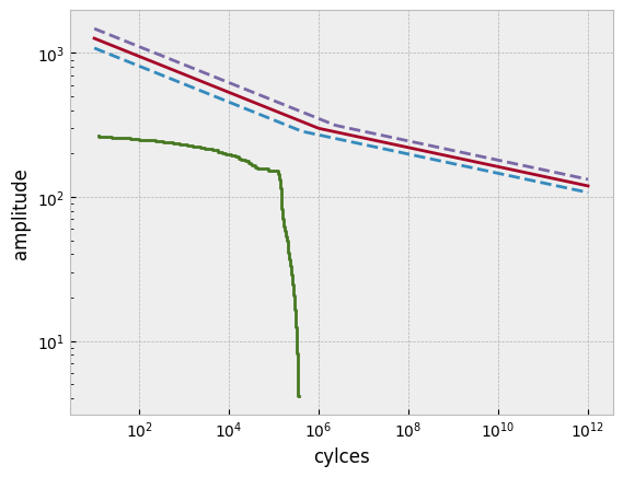
Plot the damage vs collectives
[12]:
wc = mat.woehler
cyc = pd.Series(np.logspace(1, 12, 200))
for pf, style in zip([0.1, 0.5, 0.9], ['--', '-', '--']):
    load = wc.basquin_load(cyc, failure_probability=pf)
    plt.plot(cyc, load, style)

plt.step(np.cumsum(rebinned_dict['total'][::-1]), rebinned_dict['total'].index.right[::-1])
plt.xlabel("cylces"), plt.ylabel("amplitude")
plt.loglog()
[12]:
[]
Failure Probability
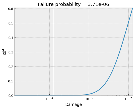
Without field scatter
In the first use case we assume, that we have the material scatter only. With that we can calculate the failure probability using the FailureProbability class.
[13]:
D50 = 0.01

damage = damage_sum_miner_haibach["total"]

di = np.logspace(np.log10(1e-1*damage), np.log10(1e2*damage), 1000)
std = pylife.utils.functions.scattering_range_to_std(mat.TN)
failprob = fp.FailureProbability(D50, std).pf_simple_load(di)

fig, ax = plt.subplots()
ax.semilogx(di, failprob, label='cdf')
plt.vlines(damage, ymin=0, ymax=1, color="black")
plt.xlabel("Damage")
plt.ylabel("cdf")
plt.title("Failure probability = %.2e" %fp.FailureProbability(D50,std).pf_simple_load(damage))
plt.ylim(0,max(failprob))
plt.xlim(min(di), max(di))
[13]:
(np.float64(9.647697093642404e-06), np.float64(0.009647697093642394))
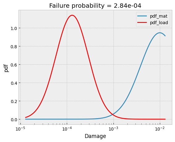
With field scatter
If we have the field scatter we can calculate the failure probability using convoluation of the probility density functions of the load and the strength.
[14]:
field_std = 0.35
fig, ax = plt.subplots()
# plot pdf of material
mat_pdf = norm.pdf(np.log10(di), loc=np.log10(D50), scale=std)
ax.semilogx(di, mat_pdf, label='pdf_mat')
# plot pdf of load
field_pdf = norm.pdf(np.log10(di), loc=np.log10(damage), scale=field_std)
ax.semilogx(di, field_pdf, label='pdf_load',color = 'r')
plt.xlabel("Damage")
plt.ylabel("pdf")
plt.title("Failure probability = %.2e" %fp.FailureProbability(D50, std).pf_norm_load(damage, field_std))
plt.legend()
[14]:
<matplotlib.legend.Legend at 0x7e42a9d1a850>
Local stress approach
FE based failure probability calculation
FE Data
[15]:
vm_mesh = pylife.vmap.VMAPImport("plate_with_hole.vmap")
pyLife_mesh = (vm_mesh.make_mesh('1', 'STATE-2')
               .join_coordinates()
               .join_variable('STRESS_CAUCHY')
               .to_frame())
[16]:
mises = pyLife_mesh.groupby('element_id')[['S11', 'S22', 'S33', 'S12', 'S13', 'S23']].mean().equistress.mises()
mises /= 150.0  # the nominal load level in the FEM analysis
#mises
Damage Calculation
[17]:
total_load = load_dict['total']
scaled_collective = total_load[total_load>0].load_collective.scale(mises)
[18]:
damage = mat.fatigue.damage(scaled_collective)
[19]:
damage = damage.groupby(['element_id']).sum()
#damage
[20]:
grid = pv.UnstructuredGrid(*pyLife_mesh.mesh.vtk_data())
plotter = pv.Plotter()
plotter.add_mesh(grid, scalars=damage.to_numpy(), log_scale=True, show_edges=True, cmap='jet')
plotter.add_scalar_bar()
plotter.show()
[21]:
print("Maximal damage sum: %f" % damage.max())
Maximal damage sum: 0.009890
Failure probability of the plate
Often we don’t get the volume of the FE data from the result file. But with pyVista we can calculate the volume (or area for 2d elements) easily:
[22]:
areas = grid.compute_cell_sizes().cell_data["Area"]
To get the failure probability we have to proceed the following steps:
get the failure probality of every element
get the probality of survival for every element
get the probality of survival for the whole component normed based on the volume (or area in 2d) of the element
get the failure probality for the whole component
[23]:
fp_per_element = fp.FailureProbability(D50, std).pf_simple_load(damage)
probability_of_survival_per_ele = 1 - fp_per_element
probability_of_survival_component = (probability_of_survival_per_ele ** (areas/areas.sum())).prod()
fp_component = 1 - probability_of_survival_component
[24]:
print('\033[1m' + "Failure probability of the component is %.2e" %fp_component)
Failure probability of the component is 3.01e-04