The WoehlerCurve data structure
The `WoehlerCurve <https://pylife.readthedocs.io/en/latest/materiallaws/woehlercurve.html>`__ is the basis of pyLife’s fatigue assessment functionality. It handles pandas objects containing data describing a Wöhler curve.
[1]:
import pandas as pd
import numpy as np
from pylife.materiallaws import WoehlerCurve
import matplotlib.pyplot as plt
The very basic Wöhler curve data
The basic Wöhler curve is a pandas.Series that contains at least three keys, * SD: the load level of the endurance limit * ND: the cycle number of the endurance limit * k_1: the slope of the Wöhler Curve
[2]:
woehler_curve_data = pd.Series({
    'SD': 300.,
    'ND': 1.5e6,
    'k_1': 6.2,
})
woehler_curve_data
[2]:
SD         300.0
ND     1500000.0
k_1          6.2
dtype: float64
[3]:
wc = WoehlerCurve(woehler_curve_data)
#wc = woehler_curve_data.woehler (alternative way of writing it)
wc.SD, wc.ND, wc.k_1
[3]:
(300.0, 1500000.0, 6.2)
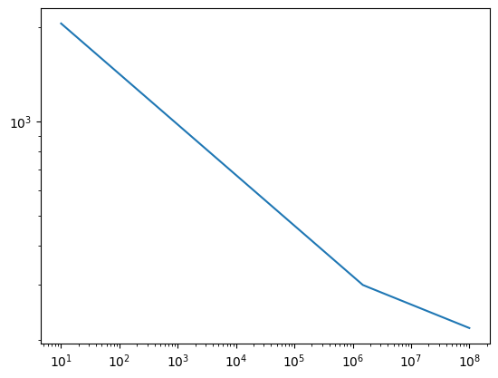
[4]:
cycles = np.logspace(1., 8., 70)
load = wc.basquin_load(cycles)
plt.loglog()
plt.plot(cycles, load)
[4]:
[<matplotlib.lines.Line2D at 0x7ff2fbbba3d0>]
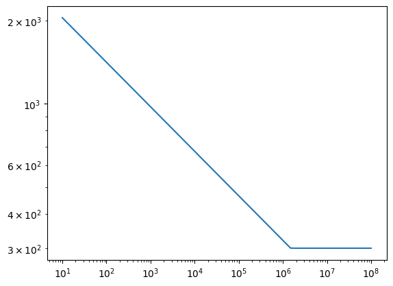
Optional parameters
The second slope k_2
You can optinally add a second slope k_2 to the Wöhler curve data which is valid beyond ND.
[5]:
woehler_curve_data = pd.Series({
    'SD': 300.,
    'ND': 1.5e6,
    'k_1': 6.2,
    'k_2': 13.3
})
plt.loglog()
plt.plot(cycles, woehler_curve_data.woehler.basquin_load(cycles))
[5]:
[<matplotlib.lines.Line2D at 0x7ff2f95bc990>]
The failure probability and the scatter values TN and TS.
As everyone knows, material fatigue is a statistical phenomenon. That means that the cycles calculated for a certain load are the cycles at which the specimen fails with a certain probability. By default the failure probability is 50%.
[6]:
woehler_curve_data.woehler.failure_probability
[6]:
0.5
You can provide values for the scattering of the Wöhler curve:
[7]:
woehler_curve_data = pd.Series({
    'SD': 300.,
    'ND': 1.5e6,
    'k_1': 6.2,
    'TS': 1.25,
    'TN': 4.0
})
Now you can then transform this Wöhlercurve to another failure probability:
[8]:
woehler_curve_data.woehler.transform_to_failure_probability(0.9).to_pandas()
[8]:
SD                     3.354102e+02
ND                     1.502105e+06
k_1                    6.200000e+00
TS                     1.250000e+00
TN                     4.000000e+00
k_2                             inf
failure_probability    9.000000e-01
dtype: float64
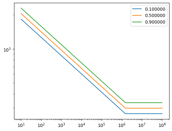
As convenience you can provide the failure probability as a optional parameter to the basquin_load() and basquin_cycles() methods.
[9]:
wc = WoehlerCurve(woehler_curve_data)
plt.loglog()
for fp in [0.1, 0.5, 0.9]:
    plt.plot(cycles, wc.basquin_load(cycles, failure_probability=fp), label="%f" % fp)

plt.legend()
[9]:
<matplotlib.legend.Legend at 0x7ff2f9329210>