The concept of stress and strength

The fundamental principle of component lifetime and reliability design is to calculate the superposition of stress and strength. Sometimes you would also say load and strength. The basic assumption is that as soon as the stress exceeds the strength the component fails. Usually stress and strength are statistically distributed. In this tutorial we learn how to work with material data and material laws to model the strength and then calculate the damage using a given load.

Material laws

The material load that is used to model the strength for component fatigue is the pylife.materiallaws.WoehlerCurve class.

First we need to importpandas and the WoehlerCurve class.

import pandas as pd
import numpy as np
from pylife.materiallaws import WoehlerCurve
import matplotlib.pyplot as plt

The material data for a Wöhler curve is usually stored in a pandas.Series. In the simplest form like this:

woehler_curve_data = pd.Series({
   'SD': 300.0,
   'ND': 1.5e6,
   'k_1': 6.2
})

Using the WoehlerCurve class can do operations on the data. To instantiate the class we use the accessor attribute woehler. Then we can calculate the cycle number for a given load.

woehler_curve_data.woehler.cycles(350.0)

array(576794.57014027)

cycles = np.logspace(1., 8., 70)
load = woehler_curve_data.woehler.load(cycles)
plt.plot(cycles, load)
plt.loglog()
plt.show()

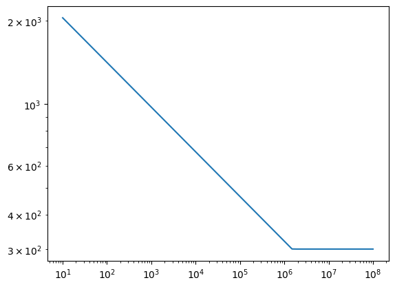
This basically means that a material of the given Wöhler curve will fail after about 577k cycles when charged with a load of 350. Note that we don’t use any units here. They just have to be consistent.

Damage sums

Usually we don’t have a single load amplitude but a collective. We can describe a collective using a python object that has an amplitude and a cycle attribute. We can do that for example with a simple pandas.DataFrame:

load_collective = pd.DataFrame({
   'cycles': [2e5, 3e4, 5e3, 2e2, 7e1],
   'amplitude': [374.0, 355.0, 340.0, 320.0, 290.0]
})

Using the pylife.strength.fatigue.damage function we can calculate the damage of each block of the load collective. Therefore we use the fatigue accessor to operate on the Wöhler data.

from pylife.strength import fatigue
woehler_curve_data.fatigue.damage(load_collective)

0    0.523107
1    0.056793
2    0.007243
3    0.000199
4    0.000000
Name: damage, dtype: float64

Now we know the damage contribution of each block of the load collective. Of course we can also easily calculate the damage sum by just summing up:

woehler_curve_data.fatigue.damage(load_collective).sum()

0.5873418943984274

Broadcasting to a FEM mesh

Oftentimes we want to map a load collective to a whole FEM mesh to map a load collective to every FEM node. For those kinds of mappings pyLife provides thepylife.Broadcaster facility.

In order to operate properly the Broadcaster needs to know the meanings of the rows of a pandas.Series or a pandas.DataFrame. For that it uses the index names. Therefore we have to set the index names appropriately.

load_collective.index.name = 'load_block'

Then we setup simple node stress distribution and broadcast the load collective to it.

node_stress = pd.Series(
    [1.0, 0.8, 1.3],
    index=pd.Index([1, 2, 3], name='node_id')
)

from pylife import Broadcaster

load_collective, node_stress = Broadcaster(node_stress).broadcast(load_collective)

As you can see, the Broadcaster returns two objects. The first is the object that has been broadcasted, in our case the load collective:

load_collective

		cycles	amplitude
node_id	load_block
1	0	200000.0	374.0
	1	30000.0	355.0
	2	5000.0	340.0
	3	200.0	320.0
	4	70.0	290.0
2	0	200000.0	374.0
	1	30000.0	355.0
	2	5000.0	340.0
	3	200.0	320.0
	4	70.0	290.0
3	0	200000.0	374.0
	1	30000.0	355.0
	2	5000.0	340.0
	3	200.0	320.0
	4	70.0	290.0

The second is the object that has been broadcasted to, in our case the node stress distribution.

node_stress

node_id  load_block
1        0             1.0
         1             1.0
         2             1.0
         3             1.0
         4             1.0
2        0             0.8
         1             0.8
         2             0.8
         3             0.8
         4             0.8
3        0             1.3
         1             1.3
         2             1.3
         3             1.3
         4             1.3
dtype: float64

As you can see, both have the same index, which is a cross product of the indices of the two initial objects. Now we can easily scale the load collective to the node stress distribution.

load_collective['amplitude'] *= node_stress
load_collective

		cycles	amplitude
node_id	load_block
1	0	200000.0	374.0
	1	30000.0	355.0
	2	5000.0	340.0
	3	200.0	320.0
	4	70.0	290.0
2	0	200000.0	299.2
	1	30000.0	284.0
	2	5000.0	272.0
	3	200.0	256.0
	4	70.0	232.0
3	0	200000.0	486.2
	1	30000.0	461.5
	2	5000.0	442.0
	3	200.0	416.0
	4	70.0	377.0

Now we have for each load_block for each node_id the corresponding amplitudes and cycle numbers. Again we can use the damage function to calculate the damage contribution of each load block on each node.

damage_contributions = woehler_curve_data.fatigue.damage(load_collective)
damage_contributions

node_id  load_block
1        0             0.523107
         1             0.056793
         2             0.007243
         3             0.000199
         4             0.000000
2        0             0.000000
         1             0.000000
         2             0.000000
         3             0.000000
         4             0.000000
3        0             2.660968
         1             0.288897
         2             0.036842
         3             0.001012
         4             0.000192
Name: damage, dtype: float64

In order to calculate the damage sum for each node, we have to group the damage contributions by the node and sum them up:

damage_contributions.groupby('node_id').sum()

node_id
1    0.587342
2    0.000000
3    2.987911
Name: damage, dtype: float64

As you can see the damage sum for node 3 is higher than 1, which means that the stress exceeds the strength. So we would expect failure at node 3.