Load Collectives and Load Histograms
From the load (stress) side pyLife provides the classes `LoadCollective <https://pylife.readthedocs.io/en/stable/stress/load_collective.html>`__ and `LoadHistogram <https://pylife.readthedocs.io/en/stable/stress/load_histogram.html>`__ to deal with load collectives. LoadCollective contains individal hysteresis loops whereas LoadHistogram contains a 2D-histogram of classes of hysteresis loops and the number of cycles with which they occur.
[1]:
import numpy as np
import pandas as pd

import matplotlib.pyplot as plt

import pylife.stress.timesignal as TS
import pylife.stress.rainflow as RF
import pylife.strength.meanstress as MS
import pylife.strength.fatigue
plt.rcParams['figure.figsize'] = [12, 7.5]
A simple load signal
Let’s take a look at a really simple load signal:
[2]:
load_signal = np.array([0., 2.0, -2.0, 1.0, -1.0, 2.0, -2.0, 1.0, -1.0, 2.0, -2.0, 1.0, -1.0, 2.0, 0.])
plt.plot(load_signal)
[2]:
[<matplotlib.lines.Line2D at 0x73c0d48739d0>]
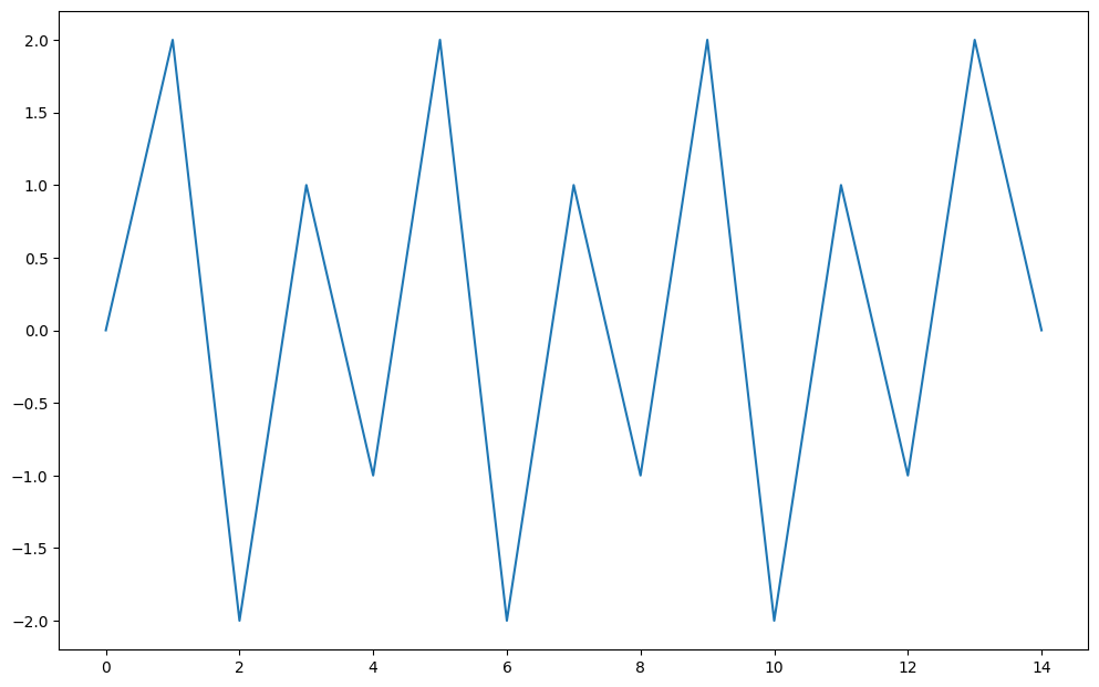
Now let’s perform a rainflow analysis.
[3]:
detector = RF.FourPointDetector(recorder=RF.LoopValueRecorder())
detector.process(load_signal)
[3]:
<pylife.stress.rainflow.fourpoint.FourPointDetector at 0x73c0d4940590>
The detector now contains the recorder which recorded the hysteresis loops for us. The simple load collective comes as a attribute of the detector:
[4]:
collective = detector.recorder.collective
collective
[4]:
| from | to | |
|---|---|---|
| 0 | 1.0 | -1.0 |
| 1 | -2.0 | 2.0 |
| 2 | 1.0 | -1.0 |
| 3 | -2.0 | 2.0 |
| 4 | 1.0 | -1.0 |
As you can see, the rainflow analysis found five hystresis loops, three from 1.0 to -1.0 and two from -2.0 to 2.0. Alternatively you can ask the recorder for a load histogram:
[5]:
histogram = detector.recorder.histogram(bins=6)
histogram
[5]:
from          to
(-2.0, -1.5]  (-1.0, -0.5]    0.0
              (-0.5, 0.0]     0.0
              (0.0, 0.5]      0.0
              (0.5, 1.0]      0.0
              (1.0, 1.5]      0.0
              (1.5, 2.0]      2.0
(-1.5, -1.0]  (-1.0, -0.5]    0.0
              (-0.5, 0.0]     0.0
              (0.0, 0.5]      0.0
              (0.5, 1.0]      0.0
              (1.0, 1.5]      0.0
              (1.5, 2.0]      0.0
(-1.0, -0.5]  (-1.0, -0.5]    0.0
              (-0.5, 0.0]     0.0
              (0.0, 0.5]      0.0
              (0.5, 1.0]      0.0
              (1.0, 1.5]      0.0
              (1.5, 2.0]      0.0
(-0.5, 0.0]   (-1.0, -0.5]    0.0
              (-0.5, 0.0]     0.0
              (0.0, 0.5]      0.0
              (0.5, 1.0]      0.0
              (1.0, 1.5]      0.0
              (1.5, 2.0]      0.0
(0.0, 0.5]    (-1.0, -0.5]    0.0
              (-0.5, 0.0]     0.0
              (0.0, 0.5]      0.0
              (0.5, 1.0]      0.0
              (1.0, 1.5]      0.0
              (1.5, 2.0]      0.0
(0.5, 1.0]    (-1.0, -0.5]    3.0
              (-0.5, 0.0]     0.0
              (0.0, 0.5]      0.0
              (0.5, 1.0]      0.0
              (1.0, 1.5]      0.0
              (1.5, 2.0]      0.0
dtype: float64
This is a bit hard to read. What you see is a pands.Series that has a two dimensional IntervalIndex as index. The histogram is all empty except the two classes from: (-2.0, 1.5] to: (1.5, 2.0] has 2.0 cycles and from: (0.5, 1.0] to: (-1.0, -1.5] has 3.0 cycles. Tose correspond to the two loops from -2.0 to 2.0 and the three loops 1.0 to -1.0.
Working with load collectives and load histograms
A load collective and a load histogram can be processed by the two classes LoadCollective and LoadHistogram. Both inherit from the common base class AbstractLoadCollective. There is the common accessor attribute load_collective that convert a pandas object with the load collective resp. load histogram data into the corresponding class.
First let’s look at a load collective. You can easily calculate the amplitude of each hysteresis loop:
[6]:
cl = collective.load_collective
cl.amplitude
[6]:
0    1.0
1    2.0
2    1.0
3    2.0
4    1.0
Name: amplitude, dtype: float64
Same for the mean stress and the R-value:
[7]:
cl.meanstress, cl.R
[7]:
(0    0.0
 1    0.0
 2    0.0
 3    0.0
 4    0.0
 Name: meanstress, dtype: float64,
 0   -1.0
 1   -1.0
 2   -1.0
 3   -1.0
 4   -1.0
 Name: R, dtype: float64)
There is also the attribute cycles:
[8]:
cl.cycles
[8]:
0    1.0
1    1.0
2    1.0
3    1.0
4    1.0
Name: cycles, dtype: float64
As you can see, the cycles are all 1.0 because we have an entry for each indivudual hysteresis loop which by definition occurs only once.
Now let’s take a look at the histogram:
[9]:
hi = histogram.load_collective
hi.amplitude, hi.meanstress, hi.R
[9]:
(from          to
 (-2.0, -1.5]  (-1.0, -0.5]    0.50
               (-0.5, 0.0]     0.75
               (0.0, 0.5]      1.00
               (0.5, 1.0]      1.25
               (1.0, 1.5]      1.50
               (1.5, 2.0]      1.75
 (-1.5, -1.0]  (-1.0, -0.5]    0.25
               (-0.5, 0.0]     0.50
               (0.0, 0.5]      0.75
               (0.5, 1.0]      1.00
               (1.0, 1.5]      1.25
               (1.5, 2.0]      1.50
 (-1.0, -0.5]  (-1.0, -0.5]    0.00
               (-0.5, 0.0]     0.25
               (0.0, 0.5]      0.50
               (0.5, 1.0]      0.75
               (1.0, 1.5]      1.00
               (1.5, 2.0]      1.25
 (-0.5, 0.0]   (-1.0, -0.5]    0.25
               (-0.5, 0.0]     0.00
               (0.0, 0.5]      0.25
               (0.5, 1.0]      0.50
               (1.0, 1.5]      0.75
               (1.5, 2.0]      1.00
 (0.0, 0.5]    (-1.0, -0.5]    0.50
               (-0.5, 0.0]     0.25
               (0.0, 0.5]      0.00
               (0.5, 1.0]      0.25
               (1.0, 1.5]      0.50
               (1.5, 2.0]      0.75
 (0.5, 1.0]    (-1.0, -0.5]    0.75
               (-0.5, 0.0]     0.50
               (0.0, 0.5]      0.25
               (0.5, 1.0]      0.00
               (1.0, 1.5]      0.25
               (1.5, 2.0]      0.50
 Name: amplitude, dtype: float64,
 from          to
 (-2.0, -1.5]  (-1.0, -0.5]   -1.25
               (-0.5, 0.0]    -1.00
               (0.0, 0.5]     -0.75
               (0.5, 1.0]     -0.50
               (1.0, 1.5]     -0.25
               (1.5, 2.0]      0.00
 (-1.5, -1.0]  (-1.0, -0.5]   -1.00
               (-0.5, 0.0]    -0.75
               (0.0, 0.5]     -0.50
               (0.5, 1.0]     -0.25
               (1.0, 1.5]      0.00
               (1.5, 2.0]      0.25
 (-1.0, -0.5]  (-1.0, -0.5]   -0.75
               (-0.5, 0.0]    -0.50
               (0.0, 0.5]     -0.25
               (0.5, 1.0]      0.00
               (1.0, 1.5]      0.25
               (1.5, 2.0]      0.50
 (-0.5, 0.0]   (-1.0, -0.5]   -0.50
               (-0.5, 0.0]    -0.25
               (0.0, 0.5]      0.00
               (0.5, 1.0]      0.25
               (1.0, 1.5]      0.50
               (1.5, 2.0]      0.75
 (0.0, 0.5]    (-1.0, -0.5]   -0.25
               (-0.5, 0.0]     0.00
               (0.0, 0.5]      0.25
               (0.5, 1.0]      0.50
               (1.0, 1.5]      0.75
               (1.5, 2.0]      1.00
 (0.5, 1.0]    (-1.0, -0.5]    0.00
               (-0.5, 0.0]     0.25
               (0.0, 0.5]      0.50
               (0.5, 1.0]      0.75
               (1.0, 1.5]      1.00
               (1.5, 2.0]      1.25
 Name: meanstress, dtype: float64,
 from          to
 (-2.0, -1.5]  (-1.0, -0.5]    2.333333
               (-0.5, 0.0]     7.000000
               (0.0, 0.5]     -7.000000
               (0.5, 1.0]     -2.333333
               (1.0, 1.5]     -1.400000
               (1.5, 2.0]     -1.000000
 (-1.5, -1.0]  (-1.0, -0.5]    1.666667
               (-0.5, 0.0]     5.000000
               (0.0, 0.5]     -5.000000
               (0.5, 1.0]     -1.666667
               (1.0, 1.5]     -1.000000
               (1.5, 2.0]     -0.714286
 (-1.0, -0.5]  (-1.0, -0.5]    1.000000
               (-0.5, 0.0]     3.000000
               (0.0, 0.5]     -3.000000
               (0.5, 1.0]     -1.000000
               (1.0, 1.5]     -0.600000
               (1.5, 2.0]     -0.428571
 (-0.5, 0.0]   (-1.0, -0.5]    3.000000
               (-0.5, 0.0]     1.000000
               (0.0, 0.5]     -1.000000
               (0.5, 1.0]     -0.333333
               (1.0, 1.5]     -0.200000
               (1.5, 2.0]     -0.142857
 (0.0, 0.5]    (-1.0, -0.5]   -3.000000
               (-0.5, 0.0]    -1.000000
               (0.0, 0.5]      1.000000
               (0.5, 1.0]      0.333333
               (1.0, 1.5]      0.200000
               (1.5, 2.0]      0.142857
 (0.5, 1.0]    (-1.0, -0.5]   -1.000000
               (-0.5, 0.0]    -0.333333
               (0.0, 0.5]      0.333333
               (0.5, 1.0]      1.000000
               (1.0, 1.5]      0.600000
               (1.5, 2.0]      0.428571
 Name: R, dtype: float64)
This might look a bit confusing as this only shows the amplitudes, meanstresses and R-values correspond to the bins of the histogram. Remember, that they were all except two empty. So let’s restrict the histogram to bins that are not empty:
[10]:
not_empty = histogram > 0.0
hi.amplitude[not_empty], hi.cycles[not_empty]
[10]:
(from          to
 (-2.0, -1.5]  (1.5, 2.0]      1.75
 (0.5, 1.0]    (-1.0, -0.5]    0.75
 Name: amplitude, dtype: float64,
 from          to
 (-2.0, -1.5]  (1.5, 2.0]      2.0
 (0.5, 1.0]    (-1.0, -0.5]    3.0
 Name: cycles, dtype: float64)
The amplitude values 1.75 and 0.75 correspond to 2.0 and 1.0. They are in the middle of the histogram bins.
A more complex example
Now let’s take a look at a more complex load collective. We use the TimeSignalGenerator to generate a load signal.
[11]:
load_signal = TS.TimeSignalGenerator(
    10,
    {
        'number': 50,
        'amplitude_median': 1.0, 'amplitude_std_dev': 0.5,
        'frequency_median': 4, 'frequency_std_dev': 3,
        'offset_median': 0, 'offset_std_dev': 0.4
    }, None, None
).query(50000)
plt.plot(load_signal)
[11]:
[<matplotlib.lines.Line2D at 0x73c0d42e2490>]
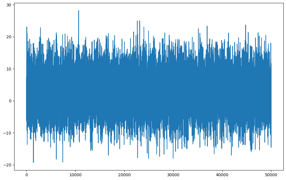
Again we perform a rainflow analysis to obtain the load histogram.
[12]:
detector = RF.FourPointDetector(recorder=RF.LoopValueRecorder())
detector.process(load_signal)

histogram = detector.recorder.histogram(64)
We can plot the histogram with a bit of processing.
[13]:
fr, to = histogram.index.levels[0], histogram.index.levels[1]
numpy_hist = np.flipud(histogram.values.reshape(len(fr),len(to)))
X, Y = np.meshgrid(fr.left, to.left)
plt.pcolormesh(X, Y, numpy_hist)
[13]:
<matplotlib.collections.QuadMesh at 0x73c0d4942270>
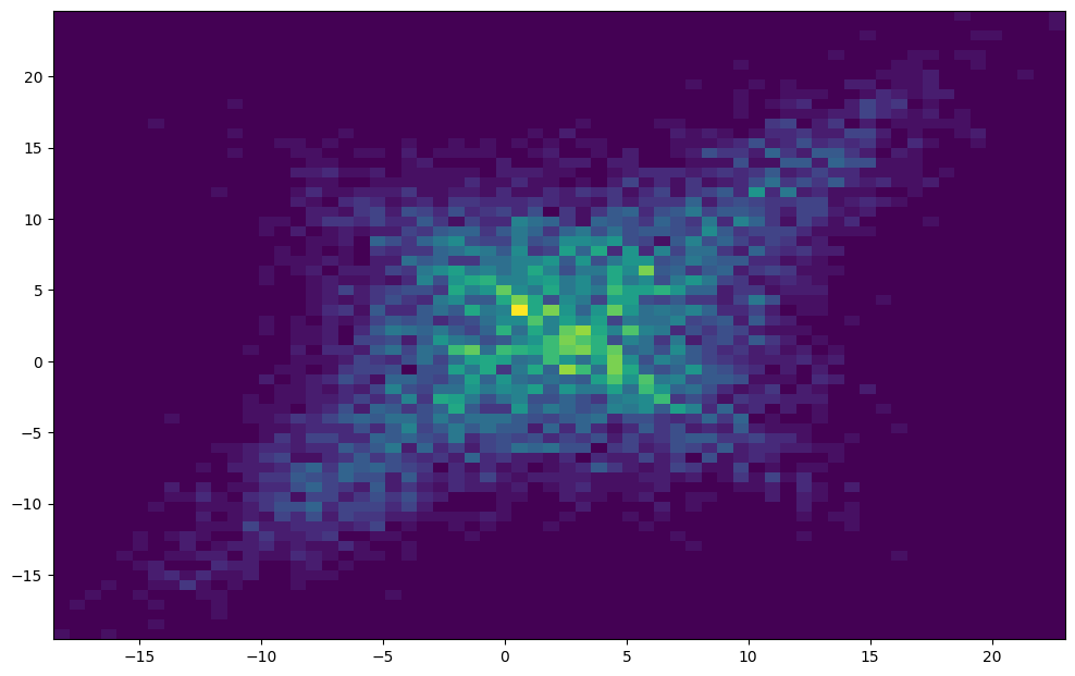
In order to use this load histogram for a damage calculation we can perform a mean stress transformation to transorm all the hysteresis loops to one given R-value.
[14]:
meanstress_sensitivity = pd.Series({
    'M': 0.3,
    'M2': 0.2
})

transformed_histogram = histogram.meanstress_transform.fkm_goodman(meanstress_sensitivity, R_goal=-1)
transformed_histogram.to_pandas()
[14]:
range                                      mean
(0.7305110777538395, 1.5138505088391896]   (0.0, 0.0]    0.0
(0.33371196647597046, 1.1170513975613157]  (0.0, 0.0]    0.0
(0.0, 0.7202522862834413]                  (0.0, 0.0]    0.0
(0.0, 0.4598862560797776]                  (0.0, 0.0]    0.0
(0.07334593627230675, 0.8566853673576518]  (0.0, 0.0]    0.0
                                                        ...
(9.371814552025914, 10.826587781184408]    (0.0, 0.0]    0.0
(8.88053946187235, 10.335312691030845]     (0.0, 0.0]    0.0
(8.3892643717188, 9.84403760087729]        (0.0, 0.0]    0.0
(7.89798928156525, 9.352762510723739]      (0.0, 0.0]    0.0
(7.406714191411654, 8.861487420570178]     (0.0, 0.0]    0.0
Length: 4096, dtype: float64
We can also plot the cumulated version of the histogram. Therefore we put the amplitude and the cycles into a dataframe.
[15]:
df = pd.DataFrame({
    'cycles': transformed_histogram.cycles,
    'amplitude': transformed_histogram.amplitude,
}).sort_values('amplitude', ascending=False)
Now we can plot the amplitude against the cumulated sum of the cycles:
[16]:
plt.plot(np.cumsum(df.cycles), df.amplitude)
plt.loglog()
[16]:
[]
